Variation Solver

What variation means

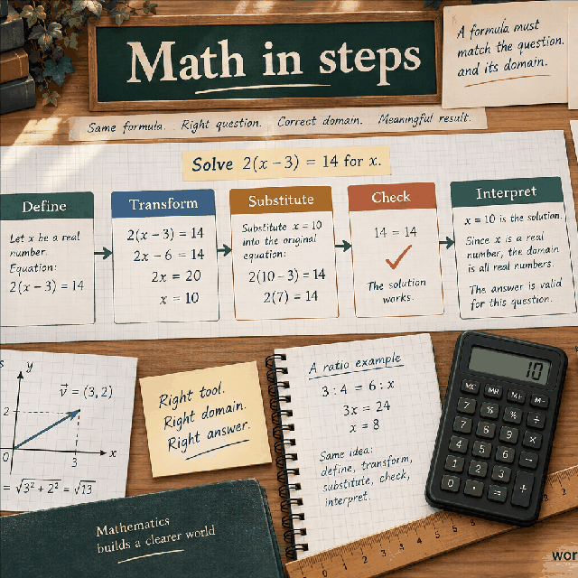
In ordinary language, two quantities vary when their values change. In algebra, variation is more specific: the changes follow a rule involving a constant. If y varies directly with x, the ratio y/x stays the same wherever that ratio is defined. If y varies inversely with x, the product xy stays the same. Joint variation extends the idea so that y depends on the product of two variables, x and z. These are not three names for the same operation. Each name describes a different invariant, and each invariant leads to a different formula.

The constant k captures the part of the relationship that is unchanged while the variables move. It is not automatically the number 1, and it is not necessarily a universal physical constant. It is a parameter for the selected model and the units used for the quantities. Once k and the relevant variable values are known, the calculator can evaluate y. If k is not known, the calculator cannot discover it from a single output field because its input contract asks you to enter k directly.

A variation statement is a model, not merely a description of two measurements. Two observations can happen to fit a direct, inverse, or joint formula without proving that the pattern will continue. A model becomes more credible when several observations give the same or nearly the same k, the units are compatible, and the relationship makes sense over the intended range. The numerical result is useful only when those modeling choices have been made deliberately.

It helps to separate three questions. First, what quantities are being related? Second, which mathematical form expresses the proposed relationship? Third, what value of k makes the form agree with the observations or definition? This calculator addresses the final evaluation once those questions have answers. Confusing model selection with calculation is a major source of incorrect variation results.

• Variation means that a relationship follows a specified rule with a fixed k.
• Direct variation preserves y/x, inverse variation preserves xy, and joint variation uses xz as the driving product.
• k belongs to the chosen model and unit system; it is not automatically universal.
• A numerical result can be correct for a model that is still a poor description of the data.

Direct, inverse, and joint models

Direct variation has the form y = kx. With k fixed, multiplying x by a factor multiplies y by that same factor. If x doubles, y doubles; if x is reduced to one third, y is reduced to one third. For a positive k, x and y have the same sign. For a negative k, they have opposite signs. When x is zero, direct variation gives y = 0, so the graph passes through the origin regardless of the value of k.

Inverse variation has the form y = k/x. Here a larger magnitude of x produces a smaller magnitude of y when k is fixed, because the product xy remains k. Doubling x divides y by two, while halving a nonzero x doubles y. The expression requires x to be nonzero. Unlike the direct graph, an inverse relationship cannot be evaluated at x = 0, and values near zero can produce very large outputs.

Joint variation has the form y = kxz. The two variables act together through their product. If x doubles while z stays fixed, y doubles. If both x and z double, y becomes four times as large. A zero in either variable makes the joint product zero. The joint model is not the same as direct variation with an extra number entered for convenience: z changes the result and must be interpreted as a genuine second variable.

The selected mode determines whether the field z has an effect. In direct mode, the calculation is y = kx. In inverse mode, it is y = k/x. In joint mode, it is y = kxz. The record keeps z as a numeric field in all modes for a consistent form, but its value is ignored in the arithmetic for direct and inverse variation. Changing z in either of those modes must not change y.

• Direct: y = kx, so y changes in the same factor as x.
• Inverse: y = k/x, so xy remains fixed and x cannot be zero.
• Joint: y = kxz, so both x and z contribute to the product.
• z is ignored in direct and inverse modes and used only in joint mode.

The constant k and its units

The units of k follow from the equation rather than from the letter itself. Suppose y has units Y, x has units X, and z has units Z. In direct variation, y = kx means that k has units Y/X. In inverse variation, y = k/x means that k has units Y times X. In joint variation, y = kxz means that k has units Y/(X times Z). Writing these units beside the formula is a simple way to catch an incompatible input or an incorrectly rearranged equation.

Changing the unit used for a variable changes the numerical value of k even when the relationship has not changed. For direct variation, if x is converted from meters to centimeters, the numerical x becomes 100 times larger, so the numerical k must become 100 times smaller to leave y unchanged. For inverse variation, the numerical k becomes 100 times larger because it is multiplied by the numerical x in the invariant xy. The formula remains the same, but the number attached to k depends on the unit convention.

Joint variation requires care with both variables. Changing the unit of x changes the numerical k in the opposite direction to that change for a direct factor, while changing the unit of z does the same. If x is represented by a value 10 times larger and z by a value 100 times larger, the numerical k must be 1,000 times smaller to produce the same y. This is why a k copied from one table cannot be reused blindly with values expressed in another unit system.

A fixed k means fixed within the scope of the model. It may describe one material, one time period, one calibration, or one chosen population. It does not promise that the underlying situation stays unchanged forever. If the process, measurement convention, or operating range changes, k may need to be refit. The calculator treats the number you enter as fixed for this calculation and has no information about whether that assumption is justified.

• Direct k units: units of y divided by units of x.
• Inverse k units: units of y multiplied by units of x.
• Joint k units: units of y divided by the product of the units of x and z.
• Changing units changes the numerical k even when the underlying relationship is unchanged.
• A fixed model constant is not automatically a permanent law of the real system.

Input contract and mode selection

The mode selector accepts exactly three choices: direct, inverse, and joint. The labels show the corresponding equations so that the selection is visible before the result is calculated. The three numeric fields are k, x, and z. Each is required to be a finite number between -1,000,000,000 and 1,000,000,000, inclusive. Decimal values and negative values are allowed. A finite number is an ordinary numeric value, not infinity and not a not-a-number value.

The field z is marked as joint only because it affects the formula only in joint mode. It is still read as a numeric input and checked against the field bounds when the handler runs. Therefore, even though changing z cannot change a direct or inverse result, z should still contain a valid finite number within the stated range. Ignoring a field in the formula does not make an invalid field value a substitute for a real numeric input.

The inverse rule has one additional condition: x must be nonzero. This includes both ordinary zero and a signed zero representation, because both represent the same point in the real-number domain. Direct and joint modes have no division by x, so x = 0 is allowed there. In joint mode, x = 0 simply makes the product and therefore y equal to zero. The value z = 0 is also valid in joint mode and has the same zero-product effect.

The output contains the calculated y and a label for the model used. The arithmetic result must remain finite; a request that would create an infinite or nonfinite output is rejected rather than displayed as if it were a meaningful measurement. Presentation is rounded to a limited number of decimal places for readability. The input bounds protect against many extreme cases, but they do not remove the need to think about tiny inverse denominators and large products.

• Mode must be direct, inverse, or joint.
• k, x, and z must each be finite and within -1e9 through 1e9.
• Inverse mode requires x!= 0; direct and joint modes allow x = 0.
• z is numerically validated in every mode but affects y only in joint mode.
• The displayed result is a rounded presentation of a finite numeric calculation.

Formulas and useful rearrangements

For evaluation, the formulas are deliberately short. Direct variation multiplies k by x. Inverse variation divides k by x. Joint variation multiplies k, x, and z. The order of multiplication in the joint expression does not matter for ordinary real numbers, but keeping the written order y = kxz makes the role of each field clear. Parentheses help when a factor is negative or fractional, for example y = (-2)(-3)(0.5).

The same formulas can be rearranged when a different quantity is unknown. From y = kx, solve for k as k = y/x when x is nonzero, or solve for x as x = y/k when k is nonzero. From y = k/x, multiply by x to obtain xy = k, so k = xy. Solving for x gives x = k/y when y is nonzero. If y = 0 and k = 0, many nonzero x values satisfy the inverse relationship, so one observation cannot identify a unique x through that rearrangement.

From y = kxz, solve for k as k = y/(xz) when both x and z are nonzero. Solving for x gives x = y/(kz) when k and z are nonzero, and solving for z gives z = y/(kx) when k and x are nonzero. Each division introduces a domain condition. If a denominator is zero, do not cancel it informally or treat a zero divided by zero as a useful result; the equation may be underdetermined or inconsistent instead.

This page evaluates y after k, x, and z have been entered. It does not provide a reverse-solving interface for k, x, or z, and it does not infer missing values. The rearrangements are still valuable because they explain how k can be obtained from observations before using the calculator. They also show why inverse and joint relationships require explicit attention to zero factors.

• Direct evaluation: y = kx; direct fitting: k = y/x when x!= 0.
• Inverse evaluation: y = k/x; inverse invariant: xy = k.
• Joint evaluation: y = kxz; joint fitting: k = y/(xz) when xz!= 0.
• Every rearrangement that divides by a quantity inherits a nonzero condition.
• The calculator evaluates y and does not solve backward for an omitted variable.

Worked direct-variation examples

Use the default direct inputs k = 5, x = 4, and z = 2. Direct mode uses y = kx, so y = 5 times 4 = 20. The value z = 2 is present but contributes nothing because the direct model has no z factor. If z is changed to -100 while k and x stay the same, the direct result remains 20. This is a useful mode check: a direct calculation should respond to k and x, not to z.

Now take k = -3 and x = 2. The result is y = (-3)(2) = -6. The negative k reverses the sign of y relative to positive x. If instead k = -3 and x = -2, then y = (-3)(-2) = 6. Direct variation follows ordinary signed multiplication. A negative result is not an error when the inputs or the chosen units permit signed quantities.

Suppose a direct relationship has k = 12 and x = 0.25. The result is y = 3. If x is then multiplied by four, from 0.25 to 1, y also multiplies by four, from 3 to 12. If x is zero, y is zero. These cases show both the scale rule and the origin behavior. The relationship is linear in x even when x is fractional or negative; there is no requirement that x be a whole number in this numeric contract.

A direct result can also be checked by dividing when x is nonzero. For k = -3, x = -2, and y = 6, the ratio y/x is 6/(-2) = -3, which recovers k. When x = 0, that ratio is unavailable even though the forward result is perfectly defined. The zero case therefore needs to be checked by substitution into y = kx rather than by forming y/x.

• k = 5 and x = 4 give y = 20 in direct mode, regardless of z.
• k = -3 and x = 2 give y = -6; k = -3 and x = -2 give y = 6.
• Multiplying x by a factor multiplies y by the same factor.
• x = 0 is valid in direct mode and always produces y = 0.
• For a nonzero x, checking y/x should recover k.

Worked inverse-variation examples

Use k = 5 and x = 4 in inverse mode. The formula is y = k/x, so y = 5/4 = 1.25. The default z = 2 does not enter this calculation. Set z to any other valid value and the result remains 1.25. The invariant check is even more direct: x times y = 4 times 1.25 = 5, which returns k.

For a signed example, let k = 24 and x = -6. Inverse variation gives y = 24/(-6) = -4. The product check is (-6)(-4) = 24. If x changes to 6 while k stays 24, y becomes 4. The sign of x matters because division by a negative number reverses the sign. If k itself is negative, the same sign rule applies: a negative k divided by a negative x gives a positive y.

Inverse scaling works in the opposite direction from direct scaling. With k = 30 and x = 5, y = 6. If x is multiplied by 3 to become 15, y is divided by 3 to become 2. If x is reduced by a factor of 2 to become 2.5, y doubles to 12. These are exact consequences of preserving the product xy, not approximate rules that depend on a particular set of numbers.

The most important edge case is x = 0. The expression k/x has no real-number value when x is zero, whether k is positive, negative, or zero. Even when k = 0, the form 0/0 is undefined rather than automatically equal to zero. The calculator therefore rejects inverse input with x = 0. Values very close to zero are allowed if they are finite, but they can produce a very large result and should be interpreted with care.

• k = 5 and x = 4 give y = 1.25 in inverse mode.
• k = 24 and x = -6 give y = -4, with xy = 24.
• Multiplying x by a nonzero factor divides y by that factor.
• z never affects an inverse result.
• x = 0 is undefined in inverse variation and is rejected.

Worked joint-variation examples

Use the default joint inputs k = 5, x = 4, and z = 2. Joint mode applies y = kxz, so y = 5 times 4 times 2 = 40. Unlike the direct and inverse examples, changing z changes the result. If z is changed from 2 to 3 while k and x remain fixed, y becomes 5 times 4 times 3 = 60. The product xz is the combined driver of the output.

Take k = 2, x = 3, and z = 4. The result is y = 2 times 3 times 4 = 24. There is no division in this model, so x and z may individually be zero. If x = 0, then y = 0 regardless of k and z. If z = 0, the same conclusion holds. A zero factor removes the whole product, just as in ordinary multiplication.

Signs are carried through all three factors. Let k = -1.5, x = -2, and z = 4. First, k times x is 3 because two negative factors make a positive product. Multiplying by z gives y = 12. If only z changes to -4, the result becomes -12 because the product now has three negative factors. This parity-of-signs view is a quick way to anticipate whether a joint result should be positive or negative.

Joint variation can look like direct variation when one variable is held fixed. If z is fixed at 2, then y = kx(2) = (2k)x, which is direct in x with an effective constant 2k. That reduced view is valid only while z remains fixed. If z changes between observations, folding it into one constant hides an important part of the model and produces a k that will not remain consistent.

• k = 5, x = 4, and z = 2 give y = 40 in joint mode.
• k = 2, x = 3, and z = 4 give y = 24.
• A zero x or zero z makes joint y equal to zero.
• The sign of y is the sign product of k, x, and z.
• Holding z fixed makes the joint relationship direct in x only for that fixed z.

Signs, zero values, and edge cases

Sign behavior follows the ordinary rules of multiplication and division. In direct mode, y is positive when k and x have matching nonzero signs and negative when their signs differ. In inverse mode, y has the sign of k divided by the sign of x, so a negative x reverses the sign. In joint mode, count the negative factors: an even number of negative factors gives a positive nonzero result, and an odd number gives a negative result. A zero factor overrides sign discussion because the product is zero.

A zero k is allowed in every mode, with one domain qualification. In direct mode, y = 0 times x = 0 for every x. In joint mode, y = 0 times x times z = 0 for every x and z. In inverse mode, k = 0 gives y = 0 for every nonzero x, but x = 0 remains invalid because the denominator is still zero. The equation's denominator condition does not disappear just because the numerator is zero.

Direct and joint formulas are defined at x = 0 because they do not divide by x. Direct x = 0 gives y = 0. Joint x = 0 gives y = 0 even when z is very large or k is negative. Joint z = 0 also gives y = 0. These results are mathematically valid under the calculator's real-number contract, though a real application may impose a separate requirement that a count, length, or rate be positive.

A finite input can still lead to a result that is too large for ordinary numeric representation, especially for inverse variation with a tiny nonzero x. Conversely, a very small result may be rounded to a visually simple value. The implementation rejects nonfinite output instead of labeling it as infinity. Treat a rejected extreme case as a signal to reconsider scale, units, or the intended domain rather than as evidence that the real-world quantity is literally infinite.

• Matching nonzero signs in direct variation produce a positive y; opposite signs produce a negative y.
• In inverse variation, a negative x flips the sign of k/x.
• In joint variation, the sign depends on the number of negative factors.
• k = 0 gives y = 0 wherever the selected formula is defined.
• Only inverse mode forbids x = 0; zero is still not a valid denominator when k = 0.

Finding k from observations

The calculator asks for k, but many variation problems begin with observed x and y values instead. Rearranging the model gives a way to calculate a candidate constant. For direct variation, use k = y/x when x is nonzero. For inverse variation, use k = xy. For joint variation, use k = y/(xz) when both x and z are nonzero. Once a candidate k has been obtained, enter it together with the relevant variables to evaluate another y.

For example, observations x = 2 and y = 14 suggest direct k = 14/2 = 7. A second observation x = 5 and y = 35 gives k = 35/5 = 7 as well, supporting the direct model over those points. In an inverse example, x = 3 and y = 8 give k = 3 times 8 = 24, while x = 6 and y = 4 give k = 6 times 4 = 24. The preserved ratio differs by model, but the consistency test is the same idea: calculate k repeatedly and compare.

For joint data, suppose x = 2, z = 3, and y = 30. Then k = 30/(2 times 3) = 5. A second observation x = 5, z = 1.2, and y = 30 also gives k = 30/(5 times 1.2) = 5. If z had been omitted from the calculation, the apparent constants would not describe the same joint relationship. Both contributing variables must be included in the invariant xz.

Zero observations need special treatment. A direct observation with x = 0 and y = 0 is compatible with every direct k, so it cannot identify k. A joint observation with x = 0 or z = 0 and y = 0 has the same limitation. An inverse observation cannot have x = 0 at all. Likewise, a nonzero x or xz paired with y = 0 implies k = 0 for the corresponding model, provided the denominator used to derive k is nonzero.

Real measurements rarely produce exactly identical constants because of noise, rounding, changing conditions, or a model that is only approximate. Several candidate k values that are close may support an approximate variation relationship, but deciding how to fit one representative value is a statistical modeling choice. This calculator does not average observations, estimate uncertainty, or perform a regression. Keep the observation table and the chosen fitting method separate from the simple evaluation step.

• Direct observations: k = y/x, requiring nonzero x.
• Inverse observations: k = xy, requiring nonzero x because the model does.
• Joint observations: k = y/(xz), requiring nonzero x and z.
• A zero-factor observation with y = 0 usually cannot identify k.
• Multiple approximate k values require a fitting decision outside this calculator.

How to check a variation model

The first check is substitution. Use the entered k, x, and, when relevant, z in the selected formula and reproduce the displayed y. For direct mode, calculate kx. For inverse mode, calculate k/x and confirm that x is nonzero. For joint mode, calculate kxz. This catches a wrong mode, a copied sign, a missing factor, or an accidental use of z in a mode where it should be ignored.

The second check uses the model's invariant. A nonzero direct observation should satisfy y/x = k. An inverse observation should satisfy xy = k. A joint observation with nonzero x and z should satisfy y/(xz) = k. The invariant is useful because it checks the relationship from a different arrangement than the forward calculation. Do not divide by a zero factor merely to create a check; use direct substitution for those cases.

The third check is a scale test. Choose a simple multiplier and predict the direction and size of change before recalculating. Direct y should change by that multiplier when x changes. Inverse y should change by the reciprocal multiplier. Joint y should follow the multiplier applied to x and the multiplier applied to z. If the numerical result violates the expected scale, inspect the mode and the factors before trusting the display.

A fourth check compares several observations rather than one result. Calculate k from each valid observation using the proper rearrangement. Exact variation should give the same k, apart from representation or measurement effects. If the constants drift systematically, the data may follow a different model, use inconsistent units, or change regime across the range. A single matching point is not enough to establish direct, inverse, or joint behavior.

• Substitute the inputs into the selected formula.
• Check the appropriate invariant: y/x, xy, or y/(xz).
• Predict a scale change before pressing calculate.
• Compare k across several valid observations.
• Use zero-factor observations by substitution, not by dividing by zero.

Scale behavior and proportional reasoning

Scale reasoning is one of the quickest ways to understand variation. In direct mode, replace x with cx, where c is any real multiplier. The formula becomes y_new = k(cx) = c(kx) = cy. Thus a positive multiplier changes the magnitude in the same proportion, while a negative multiplier also reverses the sign. A multiplier of zero sends y to zero, which is consistent with the direct domain.

In inverse mode, replace nonzero x with cx, where c is nonzero. Then y_new = k/(cx) = y/c. The output magnitude changes in the reciprocal proportion. A negative c reverses the sign, and a multiplier close to zero can make the output much larger. The excluded value c = 0 is not merely an awkward scale choice; it would create the forbidden denominator x = 0.

In joint mode, scaling x by c while keeping z fixed scales y by c, and scaling z by d while keeping x fixed scales y by d. Scaling both gives y_new = k(cx)(dz) = cd y. Doubling x and tripling z therefore makes y six times as large. If c or d is negative, the sign changes according to the product cd. This two-factor scale law distinguishes joint variation from a one-variable direct relationship.

Scale tests are also useful for planning and error detection. If a proposed direct model predicts a fourfold output when x is doubled, the mode or constant is wrong. If a proposed inverse model predicts a fourfold output when x is doubled, it may actually be a direct or power relationship. If the data are joint, changing one input while silently holding the other at a different value can make a correct model appear inconsistent.

• Direct: x -> cx makes y -> cy.
• Inverse: x -> cx makes y -> y/c for nonzero c.
• Joint: x -> cx and z -> dz makes y -> cd y.
• Negative scale factors change signs as well as magnitudes.
• Scale predictions provide a fast independent check of mode selection.

Rounding and domain assumptions

The formulas operate on the numeric values supplied to the handler, while the interface presents the result with limited decimal precision. For example, with k = 1 and x = 3 in inverse mode, the mathematical value is 1/3, while a six-place display may show 0.333333. That display is a readable approximation, not a claim that one third terminates at six decimal places. If the rounded value is reused as a new exact input, a small discrepancy can be introduced.

Rounding becomes important near a threshold or when several operations are chained. A displayed direct result of 10.000000 may come from a value that is just below or just above 10 before formatting. Inverse calculations can be especially sensitive near x = 0, where a small change in x can produce a much larger change in y. Preserve the original inputs and, when precision matters, carry more digits in the surrounding calculation than the display exposes.

The calculator assumes real numeric values. It does not know whether x and z represent lengths, times, counts, concentrations, rates, or signed coordinates. The field bounds allow negative and decimal values, even when a particular application would require nonnegative or whole-number inputs. A count may need integer rounding; a length may need to be positive; a rate may have a physical ceiling. Those are domain assumptions to state and enforce outside this generic formula evaluator.

A model can be algebraically valid but unsuitable over part of a real domain. Direct variation may only hold within a calibration range. Inverse variation may be a good approximation away from zero but fail near a saturation limit. Joint variation may omit another factor that matters in practice. The calculator checks finite numeric inputs and the inverse denominator rule; it does not validate measurement quality, scientific applicability, or extrapolation distance.

• The displayed y is rounded for readability and may not be an exact decimal representation.
• Use unrounded inputs when a small difference affects a decision.
• The generic fields permit signed real numbers, not only physically positive or integral quantities.
• Inverse results can be highly sensitive when nonzero x is close to zero.
• Numeric validation does not prove that a model is valid over the intended range.

Common mistakes

The first common mistake is choosing a formula from the word variation without identifying the type. Direct variation multiplies by x, inverse variation divides by x, and joint variation multiplies by both x and z. A result can look plausible under the wrong formula, especially when the input values are small. Write the model beside the data before entering the numbers.

Another mistake is treating k as if it had the same units in every mode. Direct k is a quotient of y units and x units. Inverse k is a product of y and x units. Joint k divides y units by the product of x and z units. Reusing a numerical k after changing centimeters to meters, hours to minutes, or one concentration scale to another can introduce a large hidden error.

Sign errors are also frequent. A negative x in inverse mode changes the sign of y, and two negative factors in a joint product restore a positive sign. Do not take absolute values unless the model explicitly calls for magnitudes. Likewise, do not treat a negative result as invalid solely because it feels unexpected; first ask whether signed variables and a signed k make it mathematically correct.

Users sometimes try to use z as a correction factor in direct or inverse mode. That changes the intended model. In those modes, z is ignored, so entering a value such as 2 does not mean that y is doubled. If z should affect the result, joint mode must be selected and the units and meaning of z must be included in k. Conversely, selecting joint mode when z is only a note adds a factor that does not belong.

Finally, do not divide by a zero observation while fitting or checking k. Direct and joint forward calculations can legitimately return y = 0, but their reverse ratios may be undefined when x or z is zero. Inverse mode rejects x = 0 from the start. Keep the direction of the calculation in mind: a forward formula may be defined in cases where a rearranged ratio is not.

• Do not confuse direct multiplication with inverse division.
• Do not use z in direct or inverse mode, and do not omit it in joint mode.
• Do not discard signs or replace signed values with absolute values without a stated reason.
• Do not reuse k after a unit change without transforming its numerical value.
• Do not infer k by dividing by a zero factor.
• Do not treat a rounded display as an exact stored value.

What the calculator does not decide

The calculator does not select direct, inverse, or joint variation from a data set. That choice requires looking at the quantities, plotting or comparing observations, considering a mechanism, and deciding what relationship is reasonable. A direct ratio can look stable over a narrow range even when a different model is more appropriate, and a few points can make an inverse product look stable by chance. The mode selector records your choice; it does not justify it.

It also does not fit k from multiple observations. You can derive candidate constants using k = y/x, k = xy, or k = y/(xz), but combining noisy candidates requires a method. An average, a weighted fit, a robust estimate, or a domain-specific calibration may each be appropriate in different situations. The page has no knowledge of measurement uncertainty, sampling design, outliers, or the cost of an error, so it cannot choose among those methods.

The tool does not attach units or enforce application-specific domain rules. It cannot tell whether a negative length is meaningful, whether a fractional item count should be rounded, whether a rate is physically possible, or whether x and z were recorded in compatible scales. It also does not decide whether a result is a prediction, an interpolation, an extrapolation, or merely an algebra exercise. Those labels depend on the data and the context supplied by the user.

Finally, a matching formula is not proof of causation or permanence. Direct, inverse, and joint forms summarize patterns; they do not explain why the pattern occurs or guarantee that it survives a change in conditions. Use the output as one transparent arithmetic step in a larger analysis. If the result informs a safety, financial, medical, engineering, or operational decision, apply the relevant review, uncertainty limits, and professional judgment separately.

• It does not infer the correct variation mode from observations.
• It does not estimate k, average noisy observations, or run a regression.
• It does not assign units, enforce positivity or integrality, or check physical plausibility.
• It does not distinguish interpolation from extrapolation.
• It does not establish causation or guarantee that k remains constant outside the stated model scope.

A practical workflow from data to result

Start by naming y, x, and, if applicable, z in words and writing their units. Decide whether the proposed relationship is direct, inverse, or joint. Ask what should stay constant: the ratio y/x, the product xy, or the relationship between y and xz. This step prevents an interface default from silently becoming a modeling decision. If the relationship came from observations, calculate k from valid nonzero factors and compare it across more than one row.

Next, confirm the input contract. Enter finite values for k, x, and z within the allowed bounds. Use signed values as measured rather than hiding a sign inside a label. In inverse mode, verify x is not zero before calculating. In direct or joint mode, decide whether zero has a meaningful interpretation in the real problem even though the algebra accepts it. In direct and inverse modes, remember that z is still validated but has no effect on y.

After the result appears, read the reported model as well as the number. Recalculate the formula by hand or with a separate substitution, check the relevant invariant when division is allowed, and perform a scale test. Compare the displayed precision with the precision of the inputs. If the result is extreme, near zero, or used near a practical limit, retain the unrounded values and document the assumptions rather than relying on the formatted display alone.

The compact summary is: select the relationship, establish compatible units, determine a defensible k, validate the denominator conditions, evaluate y, and check the result against the model. Direct variation follows y = kx, inverse variation follows y = k/x with nonzero x, and joint variation follows y = kxz. Once those distinctions are kept clear, the arithmetic is simple and the interpretation becomes much more reliable.

• Define the quantities and units before selecting a mode.
• Use the correct invariant to determine or check k.
• Enter finite k, x, and z values and respect inverse x!= 0.
• Read both y and the reported model, then verify by substitution.
• Interpret the result within the measured precision and the model's stated domain.