Elimination Method Calculator

Enter the system in standard form

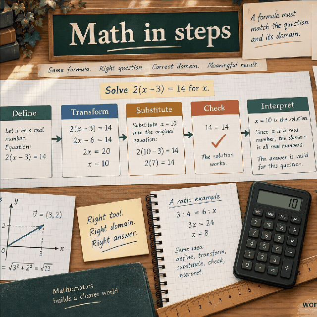
Use a₁x + b₁y = c₁ for the first equation and a₂x + b₂y = c₂ for the second. Coefficients may be negative, fractional, or zero as long as the system has a unique solution. The labels keep the left-side coefficients separate from the right-side constants.

The page is a method worksheet, so it does not ask for slope-intercept form or a graph. If an equation has a missing variable, enter zero for that coefficient. Writing the zero explicitly prevents the row from being misread during elimination.

• Keep both equations on the same standard-form side arrangement.
• Use zero for a missing x or y term.
• Do not swap a right-side constant with a coefficient.

How y is eliminated

Multiplying equation 1 by b₂ makes its y coefficient b₁b₂. Multiplying equation 2 by −b₁ makes its y coefficient −b₁b₂. Adding these scaled equations cancels y, leaving (a₁b₂ − a₂b₁)x = c₁b₂ − c₂b₁.

This is not a trick that changes the solution. Multiplying every term of an equation by the same nonzero number creates an equivalent equation, and adding equal equations preserves equality. The calculator prints the resulting coefficient so the cancellation can be inspected.

• Choose multipliers that create opposite y terms.
• Scale every term, including the right side.
• Add corresponding terms after scaling.

Recover and check y

Once x is known, substitute it into either original equation and solve for y. The returned ordered pair is then tested in both equations. A check value equal to the entered right side confirms the arithmetic for that equation.

Checking both rows matters because a copied coefficient or a missed negative sign can survive if only one equation is tested. The output keeps the two check values in the steps so the visitor can compare them directly.

• Substitute into an original equation, not a partially scaled row.
• Write the answer as (x, y).
• Check both equalities.

When the determinant is zero

The coefficient determinant a₁b₂ − a₂b₁ is the x coefficient left after eliminating y. If it is zero, the system does not have one unique intersection. The two lines may be parallel or may represent the same line, and distinguishing those cases requires comparing the full rows.

This calculator stops rather than returning an infinite or misleading decimal answer. That behavior makes the domain boundary visible; use a system-classification method when the determinant is zero.

• Zero determinant means no unique ordered-pair solution.
• Do not divide by a value that is zero or effectively zero.
• Parallel and coincident lines require classification beyond this worksheet.

Study and checking tips

Choose the variable whose coefficients are easiest to cancel when working by hand. The page always eliminates y to keep its contract consistent, but a human solver may swap variables for cleaner arithmetic. Compare the displayed multipliers with your own and then verify the ordered pair.

For a word problem, translate the story into two equations before using the tool. The calculator cannot decide whether a variable should represent people, kilograms, currency, or distance; that modeling step remains yours.

Choosing which variable to eliminate

This page consistently eliminates y because a fixed workflow makes the result easier to compare. On paper, you can eliminate x instead when its coefficients produce simpler multipliers. Both choices preserve the same intersection as long as every row operation is applied correctly.

If one coefficient is already the negative of the other, the multipliers are especially simple. If both coefficients are awkward, a least-common-multiple approach can reduce fractions before adding.

• Choose the smaller or already-opposite coefficients when working by hand.
• Scale all three entries in a row.
• The chosen variable changes the path, not the unique solution.

From a word problem to two equations

Elimination is only as reliable as the equations it receives. Define x and y in words, write the two relationships with matching units, and then place the coefficients in the six fields. A price, mixture, distance, or population problem may require a unit conversion before the algebra is ready.

After solving, translate the ordered pair back into the story. A negative quantity may signal an invalid model even when the algebraic equations are solved correctly.

• Define variables before entering numbers.
• Keep units consistent across both rows.
• Interpret the pair in the original story after checking the algebra.

Frequently asked questions

Why does the page stop at a zero determinant? Because division by the remaining x coefficient would be undefined. The rows may describe parallel lines or the same line, and a separate comparison of the constants is needed to distinguish them.

Why does a scaled equation still have the same solution? Multiplying every term by the same nonzero number creates an equivalent equality. Adding two valid equalities creates another valid equality, which is the foundation of elimination.

• Zero determinant is a classification boundary.
• Nonzero row scaling preserves the solution set.
• Check the original rows, not only the scaled rows.

See the system as two lines

Each equation in two variables describes a line when the coefficients are not both zero on the left. A unique solution is the point where the two lines intersect. Elimination is an algebraic way to find that point without first rearranging both equations into slope-intercept form, which can introduce fractions or fail for vertical lines.

The geometric view gives meaning to the determinant check. A nonzero determinant indicates that the lines are not parallel and do not coincide, so one intersection exists. A zero determinant means the coefficients do not provide a unique crossing, and the constants must be compared before choosing no solution or infinitely many solutions.

Why the determinant controls uniqueness

For the coefficient matrix with rows (a₁, b₁) and (a₂, b₂), the determinant is a₁b₂ − a₂b₁. In the elimination equation, this value multiplies x after y is canceled. If it is nonzero, division produces a single x value and substitution produces a single y value. If it is zero, that division step is not allowed.

Do not treat a very small determinant as automatically safe in a measurement problem. Exact school exercises and approximate data have different numerical behavior. This calculator stops when its unique-solution condition is not satisfied; a numerical linear-algebra workflow may need conditioning and uncertainty analysis before reporting a result.

Choose the easier variable on paper

The calculator’s contract eliminates y, but a handwritten solution can eliminate x instead. Compare the two coefficient columns and choose the one that needs smaller or already-opposite multipliers. The final ordered pair should be the same when both paths are performed correctly, so the choice is a convenience rather than a change in the mathematics.

When a teacher asks specifically for elimination of y, follow that instruction even if x looks shorter. When solving a practical model, fewer fractions usually means fewer opportunities for transcription error. Keep the chosen variable visible in the work so a reviewer understands why the scaling factors look the way they do.

Scale every term in the row

A row operation multiplies the x coefficient, y coefficient, and right-side constant by the same nonzero multiplier. Scaling only the variable coefficient breaks the equation and leads to a plausible-looking but incorrect intersection. Write the multiplier beside the entire equation before distributing it.

For example, multiplying 2x + y = 7 by −2 gives −4x − 2y = −14. The right side is part of the equality, not an afterthought. The calculator displays the scaling information so the visitor can check that the constants were transformed along with the left side.

• Multiply x, y, and the constant together.
• Keep the multiplier visible.
• Never divide a single term in isolation.

Use least common multiples to reduce clutter

If the y coefficients are 6 and 4, one hand strategy is to scale the first row by 2 and the second by −3. The new y coefficients are 12 and −12, so adding cancels them. Choosing the smallest convenient common multiple keeps the intermediate constants smaller and reduces the chance of a sign mistake.

Fractions can also be valid. Multiplying by a common denominator first may make a system easier to read, but it is not required if the calculator accepts the values. Whatever route you choose, verify the final pair in both original equations rather than trusting a simplified intermediate row.

A second worked system

Consider 3x + 2y = 16 and 5x − 2y = 8. The y coefficients are already opposites, so adding the rows produces 8x = 24 and x = 3. Substituting into the first row gives 9 + 2y = 16, so y = 3. The ordered pair is (3,3), and both original rows evaluate to their stated constants.

This example shows why the addition step is the heart of the method. No variable was guessed and no graph scale was selected. The coefficients were arranged so one dimension disappeared, leaving a one-variable equation that could be checked and then reversed through substitution.

Distinguish parallel from coincident lines

When the determinant is zero, compare the full equations rather than stopping at the phrase parallel. If the coefficient ratios and constant ratio agree, both rows describe the same line and infinitely many points satisfy the system. If the coefficient ratios agree but the constants do not, the lines are distinct and parallel, so no point satisfies both.

A ratio test can be awkward when a coefficient is zero. Comparing cross-products or reducing the rows is safer than dividing by a value that may be zero. The calculator intentionally focuses on unique ordered pairs; use a classification worksheet for these two zero-determinant cases.

Signs are the main elimination trap

A negative multiplier changes every sign in the row. It is easy to create opposite y coefficients correctly and then forget that the x coefficient and constant changed too. Write the scaled rows on separate lines and add columns in a fixed order: x coefficient, y coefficient, constant.

If the calculated x has the wrong sign, check the right-side subtraction as well as the left-side coefficients. Substitute the result into both original equations. A pair that satisfies one row may still reflect an arithmetic error that happened to cancel in the other row.

• Scale signs across the whole row.
• Add matching columns only.
• Use both original equations as checks.

Word problems require modeling before elimination

A calculator cannot decide what x and y represent. In a ticket problem they might be adult and student tickets; in a mixture problem they might be amounts of two solutions; in a distance problem they might be rates or times. Define the variables in words, translate each relationship, and check the units before entering six coefficients.

After solving, interpret the pair in the story. A negative number, a non-integer count, or a value outside a stated capacity can indicate that the algebra solved a model that was not appropriate for the real question. Keep the equation solution and the story’s feasibility check as separate steps.

Keep units consistent

The terms added in an equation must represent compatible quantities. If one equation uses cents and another uses dollars, convert before elimination. If a distance is in kilometres and a rate is in miles per hour, the model needs a conversion before the coefficients are meaningful. The calculator performs number operations, not hidden unit conversions.

Write the unit beside each variable and constant during setup. A solution can satisfy the numeric equations while still answering the wrong real-world question if the units were mixed. This is one reason the article treats model translation as part of a reliable workflow rather than as optional context.

Substitution is the independent check

Elimination finds one variable and substitution recovers the other. Substitution back into both original equations is also an independent verification because it uses the initial relationships rather than only the scaled rows. For a pair (x, y), calculate a₁x + b₁y and a₂x + b₂y and compare each with c₁ and c₂.

If the checks differ by a small amount in a decimal system, decide whether that is ordinary display rounding or a meaningful residual. For exact classroom integers, a mismatch is an error. Report the check values and the precision rule instead of hiding a discrepancy behind a rounded ordered pair.

Exact values versus approximate measurements

In textbook systems, coefficients are often exact integers or fractions. In a measured model, coefficients can be estimates and the intersection can inherit uncertainty. The calculator returns a numeric solution under the entered values; it does not calculate confidence intervals, measurement error, or sensitivity to coefficient changes.

If the inputs come from data, vary one coefficient within a plausible range and observe how the pair moves, or use a method designed for uncertainty propagation. Keep more precision internally than you display, and label the final answer as a model result rather than an exact physical truth.

The matrix view explains the same method

The system can be written as a two-by-two coefficient matrix multiplied by the vector (x, y), equal to the constants vector. Elimination is a row-operation approach to transforming that matrix into a form where one variable is isolated. The calculator uses the six scalar fields so the process remains understandable without requiring matrix notation.

This connection helps when moving to larger systems. Gaussian elimination generalizes the same idea, while this page deliberately limits the contract to two equations and two unknowns. Do not infer that a unique pair from this tool solves a model with additional variables or constraints that were not entered.

Use graphs as a visual explanation

A graph of the two lines can make the ordered pair intuitive. Plot each original equation, mark the intersection, and use the calculator’s pair as the coordinates. The graph is a visual companion, not the source of the numeric precision, because a screen scale can make nearby lines appear to meet or hide a small difference.

For a vertical line, slope-intercept form is inconvenient but standard form and elimination still work. This is a practical advantage of keeping the equations in coefficient form. Use the graph to communicate geometry and the substitution checks to validate arithmetic.

Create a review table

A strong solution record can use columns for original row, multiplier, scaled x coefficient, scaled y coefficient, scaled constant, and final check. Add the determinant and the ordered pair at the top. This makes a tutor or classmate able to trace the result without reconstructing hidden mental steps.

For a word problem, add variable definitions, units, and a feasibility note. For a decimal model, add input precision and residual tolerance. A table is not extra decoration; it separates the equation operation from the interpretation and gives each possible error a visible location.

Choose the next method deliberately

After solving a unique system, the next question may be graphing the lines, checking a word-problem constraint, solving a system with three variables, or comparing how the answer changes when a coefficient changes. Link to the relevant next calculator with descriptive text rather than sending every visitor to an undifferentiated tool list.

If the determinant is zero, continue to system classification. If the model has uncertainty, continue to sensitivity or regression methods. If the variables are nonlinear, use a nonlinear solver. The best internal path follows the mathematical question that remains, not the page that happens to be nearby.

Near-parallel lines need caution

A nonzero determinant guarantees a unique algebraic pair, but a very small determinant can make the pair sensitive to small changes in measured coefficients. The calculator uses the entered values exactly as numbers and does not estimate that sensitivity. In a data-driven model, perturb the inputs or use a numerical-analysis method before making a strong practical claim.

This distinction is useful for students too. A system can have one exact intersection while its rounded graph appears parallel. Trust the coefficient calculation and substitution checks for the stated inputs, then label approximate applications with the precision supported by their measurements.

Check the solution against story constraints

After the algebraic pair is verified, apply constraints from the original problem. Ticket counts may need to be whole and nonnegative, mixture amounts may need to stay within available containers, and a budget variable may have an upper limit. These restrictions are not encoded in six unrestricted real-number fields.

Keep an infeasible pair visible as a modeling warning rather than silently replacing it. The equations may be inconsistent with the story, the units may have been mixed, or a condition may have been omitted. A clear feasibility note tells the reader what must be revised before using the result.

Use an audit trail for teaching

For a worked lesson, save the original rows, the chosen multipliers, the scaled rows, the canceled column, the reduced equation, the solved variable, the back-substitution, and both checks. This order mirrors the logic of elimination and makes each transformation reviewable. A student can correct one row without discarding the entire solution.

For a technical worksheet, add input source, units, precision, and a note about uniqueness. The record can then be read by someone who did not watch the calculation happen. That is the difference between a useful method result and an unexplained pair copied into a report.

Final elimination checklist

Before accepting the pair, confirm standard-form placement, missing coefficients entered as zero, consistent units, the chosen variable, row multipliers, opposite elimination coefficients, the scaled right sides, a nonzero determinant, and substitution checks in both original equations. Keep the ordered pair separate from any story interpretation.

Then label the result as a unique algebraic solution, a model scenario, or an approximate measurement. If the determinant is zero, do not invent a decimal answer; classify the system with an appropriate method. A transparent elimination record teaches the operation, exposes the assumptions, and gives the visitor a safe next step.