Derivative at a Point (Central Difference)

What a derivative at a point means

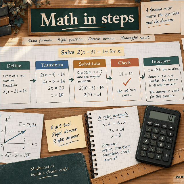
A derivative is a local rate of change. If y = f(x), the derivative f'(a) tells you how much y is changing per unit of x at the input x = a. On a graph, it is the slope of the tangent line at the point (a, f(a)). The word local is important: a derivative describes behavior arbitrarily close to a point, not an average change over a wide interval. A curve can rise overall while having a negative derivative at one location, or it can have a positive derivative that is becoming smaller as the curve flattens.

The exact derivative is defined by a limit of difference quotients as the spacing approaches zero. In practice, a calculator cannot usually evaluate a literal zero-width interval. It instead uses a small positive h and samples the function at a - h and a + h. Those two sample locations are equally far from a. The central-difference result is the slope of the secant line joining the samples, used as an approximation to the tangent slope at their midpoint.

This page does not require you to enter a, f(a), or a formula for f. The midpoint and the two function values are assumed to be known before you use the calculator. If the values were taken at locations that are not actually symmetric around the intended point, the returned number is a slope over those supplied locations, not necessarily a central estimate at the point you had in mind. Keeping the sample locations in your notes protects against that easy-to-miss mismatch.

The result is therefore best read as an estimate with a stated spacing, not as an unexplained exact derivative. A result of 4 means that, under the supplied pair of values and step size, the local change is estimated at 4 output units for each input unit. Whether that is a good estimate depends on how the values were generated and on what happens between the two sample locations.

• A derivative is a local rate of change at an input point.
• A central difference uses two values equally far from the point.
• The result is a secant slope used to estimate a tangent slope.
• The calculator assumes that your two values really correspond to a - h and a + h.

The central-difference formula

The calculator evaluates f'(a) approximately equal to (f(a + h) - f(a - h)) / (2h). The numerator is the change in function value between the upper-side and lower-side samples. The denominator is the full horizontal distance between those samples: from a - h to a + h is a distance of 2h, not h. Dividing by 2h gives a slope with the correct scale.

The order of subtraction matters. The upper value f(a + h) is placed first, and the lower value f(a - h) is subtracted from it. If the function rises as x increases, the numerator is usually positive and the estimated derivative is positive. Reversing the values would reverse the sign and would no longer represent the stated quotient. The h field is a distance from the midpoint to either sample, so it remains positive even when the input coordinate a or either function value is negative.

Symmetry is the defining feature of this difference. A forward difference compares f(a + h) with f(a), while a backward difference compares f(a) with f(a - h). The central version places the target point between the samples, so the first-order effects on the two sides cancel for a sufficiently smooth function. This is why it often gives a more accurate estimate than a one-sided quotient at the same h, although it requires two nearby values and can be more sensitive to noise when h is made very small.

The handler performs the arithmetic directly from the three numbers. It does not fit a curve to a larger table, smooth the inputs, estimate uncertainty, or search for a better h. Its output includes the numeric derivative and calculation steps so that you can see the subtraction and the denominator. Use those steps to check the sign, the factor of 2, and the unit interpretation before drawing a conclusion.

• Numerator: upper-side function value minus lower-side function value.
• Denominator: 2h, the full distance between the samples.
• The sample midpoint is a, because the locations are a - h and a + h.
• The method trades one-sided bias for a symmetric two-point estimate.

Inputs and validation rules

The f(a - h) field accepts the function value at the lower input location. It must be a finite number from -1,000,000,000,000 through 1,000,000,000,000, inclusive. The f(a + h) field has the same range and represents the value at the upper input location. Negative values, zero, and positive values are all allowed because a function value can have any of those signs under the calculator's general numeric contract. The fields expect numbers, not expressions such as 2 + 3 or labels with units attached.

The Step size h field accepts a finite positive number greater than zero and no greater than 1,000,000,000. The lower boundary is open: h = 0 is invalid because the quotient would divide by zero and because the two sample locations would collapse into one location. Negative h is also rejected. A positive h is enough to identify which supplied value is the lower-side sample and which is the upper-side sample; you do not need to encode direction in the step size.

The bounds are validation limits, not claims about the natural size of a derivative problem. A function value at exactly either numeric endpoint is accepted, while a value outside the range, a blank value, a nonnumeric value, infinity, or not-a-number is rejected. The same finite-number rule applies to h. The calculator does not silently change a value to the nearest allowed endpoint. If a value is rejected, fix the source or rescale the problem deliberately rather than treating a substituted value as the original measurement.

A valid input can still yield a poor estimate. The validator can confirm that three numbers are finite and bounded, but it cannot know whether the values came from the same function, whether the locations are symmetric, whether the function is smooth, or whether the step is appropriate. It also checks that the arithmetic result remains finite. Passing validation means the numerical contract was met; it does not certify mathematical accuracy or physical measurement quality.

• Both function-value fields accept finite numbers from -1e12 to 1e12, inclusive.
• h must be finite, strictly positive, and no greater than 1e9.
• Zero, negative, nonfinite, malformed, blank, and out-of-range inputs are invalid.
• Validation checks numbers and bounds, not the truth of the supplied function values.

Units and the meaning of the slope

A derivative carries a unit relationship even when the calculator displays only a bare numeric value. If x is measured in seconds and f(x) is measured in meters, then f'(x) is meters per second. If x is in meters and f(x) is in kilograms, the derivative is kilograms per meter. The numerator has the output unit, h has the input unit, and division by 2h produces output units per input unit. This dimensional check is one of the quickest ways to catch a mistaken input.

The page has no unit selector and cannot convert prefixes for you. You must use one consistent input unit for h and for the locations where the two values were evaluated. If the samples are 2 milliseconds apart in total, the central step h is 1 millisecond, or 0.001 seconds. Entering h as 1 while interpreting the function values as seconds would scale the derivative by a factor of 1000. Likewise, if the function values are reported in centimeters, do not describe the result as meters per second unless you convert the numerator first.

Suppose a measured position is 12.4 meters at time a - h and 12.8 meters at time a + h, with h = 0.2 seconds. The estimate is (12.8 - 12.4) / 0.4 = 1 meter per second. If the same position difference were entered as 40 centimeters, the numeric result would be 100 centimeters per second, which is the same rate after conversion. The arithmetic is consistent only when the unit description travels with the values.

A dimensionless function can still have a unit-bearing derivative. For example, a probability, a proportion, or a normalized score may have no physical unit, but its derivative with respect to seconds is per second. Conversely, if both x and f(x) are counts of the same kind, the ratio may be described as count per count, though the practical interpretation depends on the context. The calculator reports the number; you supply the honest unit label.

• Derivative units are output units divided by input units.
• h must use the same input-unit convention as the sample locations.
• Convert milliseconds, centimeters, percentages, and other prefixes before entry when needed.
• A dimensionless output can still have units such as per second or per meter.

Why symmetry improves the approximation

The accuracy advantage of the central difference can be seen by expanding the function around a. For a smooth function, f(a + h) can be written as f(a) + h f'(a) + h^2 f''(a)/2 + h^3 f'''(a)/6 plus higher-order terms. The matching expansion for f(a - h) is f(a) - h f'(a) + h^2 f''(a)/2 - h^3 f'''(a)/6 plus higher-order terms. The signs of the odd-power terms change across the midpoint, while the even-power terms keep their signs.

Subtract the lower expansion from the upper expansion. The two copies of f(a) cancel. The terms involving f''(a) also cancel because they have the same sign on both sides. The first derivative terms add to 2h f'(a), and the leading remaining contribution comes from the third derivative term. Dividing by 2h leaves f'(a) plus a leading error proportional to h^2, rather than an error proportional to h.

This is commonly described as second-order truncation behavior. In a smooth region, reducing h by a factor of two can reduce the leading approximation error by roughly a factor of four, provided arithmetic rounding and measurement noise have not become dominant. That condition matters. The limit argument describes the behavior of the mathematical formula with accurate function evaluations; it does not promise that a smaller entered step always improves a real set of rounded or noisy values.

The cancellation also explains why the central method is exact for every linear function and for every quadratic function when the supplied function values are exact. A quadratic has a constant second derivative and no third-derivative contribution, so the symmetric secant slope equals the tangent slope at the midpoint. For higher-degree functions, the estimate is generally close rather than exact, with the difference controlled by local curvature changes and the chosen spacing.

• Symmetric samples cancel the constant and even second-order terms in the expansion.
• For a smooth function, the leading central-difference truncation error is proportional to h^2.
• Halving h can reduce truncation error by about four when other errors are small.
• Exact function values make the method exact for linear and quadratic functions.

Worked example: the catalog default

The default-style inputs are f(a - h) = 7.2, f(a + h) = 8.8, and h = 0.2. These values say that the function is 7.2 at the lower sample and 8.8 at the upper sample, with each sample 0.2 input units from the midpoint. The full distance between the samples is therefore 2h = 0.4 input units.

First find the change in function value: 8.8 - 7.2 = 1.6. Next divide that change by the full horizontal distance: 1.6 / 0.4 = 4. The calculator returns an estimated derivative of 4. The result is positive because the upper-side value is larger than the lower-side value. It means the central secant slope is 4 output units per input unit under the units you assign to the fields.

The number 4 is not obtained by dividing 1.6 by h alone. Doing 1.6 / 0.2 would give 8 and would treat the distance between the samples as half its actual value. The step h describes one side of the interval, while the numerator spans both sides. Writing 2h before substituting numbers makes this factor-of-two error easier to avoid.

The example alone cannot prove the exact derivative at a. Many different functions can pass through the two supplied points and have different slopes at the midpoint. If you know the original formula, compare this estimate with its analytic derivative. If you have a larger table, compute several neighboring estimates and examine whether they agree as the step changes.

• Difference in values: 8.8 - 7.2 = 1.6.
• Full sample spacing: 2 x 0.2 = 0.4.
• Central estimate: 1.6 / 0.4 = 4.
• Interpret 4 using the output-unit per input-unit relationship.

Worked example from a known function

Consider f(x) = x^2 and estimate the derivative at a = 3 with h = 0.1. The calculator does not receive the formula or a, so compute the two required values first. The lower location is 2.9, giving f(2.9) = 8.41. The upper location is 3.1, giving f(3.1) = 9.61. Enter fMinus = 8.41, fPlus = 9.61, and h = 0.1.

The central quotient is (9.61 - 8.41) / (2 x 0.1) = 1.20 / 0.20 = 6. The exact derivative of x^2 is 2x, which is 6 at x = 3, so this example agrees exactly. That agreement is expected: the central difference is exact for a quadratic when the function values are evaluated without rounding. It is a useful test of both the input order and the denominator.

Now imagine that the same values were rounded too aggressively before entry. If 8.41 were recorded as 8 and 9.61 as 10, the calculator would return (10 - 8) / 0.2 = 10, even though the underlying derivative is 6. The arithmetic would be correct for the rounded inputs, but the inputs would no longer represent the function closely enough. Preserve useful digits in the function values, especially when their difference is small compared with their individual sizes.

This example also shows why a is not needed for the final arithmetic but is still needed for interpretation. Without a, the calculator cannot label the location of the estimate or check that the supplied values came from x = 2.9 and x = 3.1. Keep a and the sample locations in the surrounding calculation record even though only fMinus, fPlus, and h are entered here.

• For x^2 at a = 3 and h = 0.1, the samples are 8.41 and 9.61.
• The central quotient is (9.61 - 8.41) / 0.2 = 6.
• The exact derivative 2a is also 6, as expected for a quadratic.
• Rounded function values can destroy an otherwise accurate difference.

Worked example: seeing truncation error

Use f(x) = x^3 at a = 2 with h = 0.5. The lower sample is x = 1.5, where f is 3.375. The upper sample is x = 2.5, where f is 15.625. The central estimate is (15.625 - 3.375) / (2 x 0.5) = 12.25 / 1 = 12.25. The exact derivative is 3x^2, which equals 12 at x = 2, so the central result is high by 0.25.

For this cubic, the third derivative is 6 everywhere. The leading central truncation term is h^2 f'''(a) / 6, which becomes 0.25 when h = 0.5. In this special example the expression gives the complete error, not only an approximation to it. It demonstrates that symmetry removes the first-order error but does not make every nonlinear function exact.

Repeat the same calculation with h = 0.25. The locations are 1.75 and 2.25, with function values 5.359375 and 11.390625. Their difference is 6.03125, and the full spacing is 0.5, so the estimate is 12.0625. The error is now 0.0625, one quarter of the previous 0.25 error. This is the expected fourfold reduction when h is halved and the values are exact.

The example is a model-based check, not a promise about every dataset. If the function values were measured with enough noise, the h = 0.25 result could be less trustworthy than the h = 0.5 result even though its truncation error is smaller. A useful comparison always considers both approximation error and value quality.

• For x^3 at a = 2 and h = 0.5, the estimate is 12.25 instead of 12.
• With h = 0.25, the estimate becomes 12.0625.
• Halving h reduces this cubic's truncation error from 0.25 to 0.0625.
• The improvement assumes exact function evaluations and no measurement noise.

How to choose a useful h

There is no universal best value for h. A useful step is small enough that the function behaves nearly linearly over the interval from a - h to a + h, yet large enough that the change in function value is not hidden by rounding or noise. The right scale depends on the units, the size of a, the curvature of f, the precision of the evaluation process, and the purpose of the estimate. A value that is sensible for seconds may be absurd for meters or for a normalized coordinate.

Start by identifying the scale of the input and the local feature you need to resolve. If a function changes rapidly over a narrow region, a large h can average across meaningful structure. If it changes slowly and the values are reported with only a few decimal places, an extremely small h can make the subtraction produce mostly numerical or measurement artifacts. The field's lower boundary is only greater than zero; it does not tell you which positive value is scientifically appropriate.

When several values are available, compute a short h-sweep. Try a central step, then a value about half as large and one about twice as large, while recomputing the two function values at the matching locations. If the estimates move toward a stable plateau as h decreases, truncation error may be shrinking. If they become erratic, the difference is likely being dominated by rounding, noise, or an evaluation limit. If they change smoothly but never settle, the interval may still be too wide or the function may not be smooth enough.

Keep h tied to the sample generation process. If the values come from a table with a fixed grid, you may be limited to steps that place samples on that grid. If the data are collected at irregular times, the central formula cannot be used honestly unless you have values at equal distances from the target or you adopt a different method. Do not claim a smaller h merely by changing the denominator while reusing values from the old locations; the numerator must correspond to the same h.

A report should state how h was selected and whether it was tested. Saying only that h was small is not reproducible. State its numeric value and unit, the two sample locations, the precision of the values, and any comparison with nearby h values. That context lets another reader tell whether the estimate reflects local behavior or an arbitrary spacing choice.

• Choose h relative to the input scale and the local variation of the function.
• Do not assume the smallest positive h is the most accurate.
• Recompute f(a - h) and f(a + h) whenever h changes.
• Compare several h values and look for stability rather than one attractive number.
• Record the numeric h, unit, sample locations, and selection reason.

Truncation error and local curvature

Truncation error is the error caused by replacing a limiting derivative with a finite spacing. It is not a typo or a failure of the calculator. Even if fMinus and fPlus are evaluated with infinite precision, the secant slope across a nonzero interval may differ from the tangent slope at its midpoint. For the central difference and a sufficiently smooth function, the leading term is proportional to h^2 and involves the third derivative nearby.

The sign of truncation error depends on how the local slope changes. A cubic example may produce an overestimate for one curvature pattern and an underestimate for another. Looking only at whether the function is increasing is not enough to predict the error. The derivative can be positive while the third-derivative contribution is positive or negative. This is why comparing estimates across h values is more informative than applying a generic rule such as always rounding the result down.

If the function is exactly linear over the interval, the secant and tangent slopes agree. If it is quadratic, the symmetric slope agrees at the midpoint even though the graph is curved. For a higher-order function, a small interval usually makes the local curve look more nearly quadratic, reducing the central estimate's truncation component. The interval still must lie in a region where the function is defined and where a derivative is meaningful.

A large h can conceal a local feature. For example, a steep rise followed by a flattening may have a moderate average secant slope even when the derivative at the midpoint is much larger or smaller. The central quotient does not know what happens between its two endpoints. It summarizes the two values you supplied, so the burden of checking local behavior remains with the person who selects the samples.

• Truncation error remains even when the two function values are exact.
• Central truncation error is usually second order in h for a smooth function.
• Linear and quadratic behavior is especially favorable for the symmetric quotient.
• A wide interval can average over a feature that matters at the midpoint.

Rounding error, cancellation, and noise

The numerator f(a + h) - f(a - h) can be much smaller than either function value. When two large, nearly equal numbers are subtracted, the shared digits cancel and the remaining difference may have relatively poor precision. Dividing that small difference by 2h then exposes the loss. This is a central numerical tradeoff: reducing h often lowers truncation error, but it also makes the function values more similar and can magnify errors in their difference.

Suppose each supplied function value contains an additive error, written ePlus and eMinus. The derivative estimate inherits the error (ePlus - eMinus) / (2h). If the errors happen to have opposite signs, their effect can add. If they happen to be similar, some error can cancel. You cannot safely assume either outcome for independently rounded or measured values. The smaller h becomes, the larger the same value-error contribution becomes in the derivative.

For independent measurement errors with standard deviations sigmaPlus and sigmaMinus, a simple uncertainty model gives a derivative standard deviation of approximately square root of (sigmaPlus squared plus sigmaMinus squared) divided by 2h. If both uncertainties are the same sigma, this becomes sigma divided by square root of 2 times h. The calculator does not receive uncertainty fields and does not compute this interval, but the relationship explains why a noisy experiment can prefer a wider h than an exact formula evaluation.

Noise can also be structured rather than random. A sensor drift, a calibration offset, a changing sampling delay, or a rounded lookup table may affect the two sides differently. Repeating the same central quotient does not remove a systematic error. If you smooth or fit a curve before differentiating, you may obtain a more stable estimate, but you have changed the method and introduced assumptions that should be documented separately from this two-value calculation.

The practical goal is balance. Choose an h for which the numerator is large enough to resolve with the available precision but the interval is still local enough for the derivative question. Report fewer digits when the inputs do not support the displayed precision. A long decimal result is a property of arithmetic formatting, not proof that the underlying rate is known to the same number of places.

• Subtracting nearly equal values can lose significant digits.
• Input errors are divided by 2h, so smaller h amplifies their effect.
• Independent noise uncertainty generally grows as h becomes smaller.
• Smoothing or fitting data is a separate modeling step, not part of this handler.
• Match reported digits to the precision and repeatability of the inputs.

Using h-sweeps to diagnose the tradeoff

An h-sweep is a practical diagnostic rather than a new formula. Select a target point and calculate central estimates at several decreasing positive steps. For each step, regenerate or retrieve the values at the corresponding symmetric locations. Place h and the resulting derivative in a table. A smooth drift toward one value suggests that finite-interval truncation is still changing the answer. A noisy scatter suggests that rounding or measurement error has become important.

For exact smooth function evaluations, the difference between the estimate at h and the estimate at h/2 often shrinks by about four when the central method's second-order term dominates. If the changes follow that pattern, the estimates may be in the asymptotic truncation region. If halving h changes the answer by a factor that is much smaller than expected and then begins to produce random-looking digits, the precision floor may have been reached. Neither pattern is a formal proof, but both are useful evidence.

Two central estimates can also support a Richardson-style correction when the leading error really behaves like C h^2. If D(h) is the estimate at h and D(h/2) is the estimate at half the step, a refined value can be formed as (4D(h/2) - D(h)) / 3. This is an additional calculation, not an output of this page, and it can make noise worse because it combines two estimates. Use it only when smoothness and repeatability justify the assumed error model.

If the data are noisy, the best-looking h may be an application choice rather than a mathematical optimum. A wider step can average over noise only if the function values themselves come from an appropriate averaging process; simply using endpoints farther apart changes the local question. Keep the h-sweep as evidence, identify the stable range if one exists, and explain why the selected step matches the resolution needed by the application.

• Recompute both function values for every h in a comparison table.
• A fourfold change pattern can indicate second-order truncation dominance.
• Richardson correction assumes a stable h^2 error model and is not built into this page.
• Noise, drift, and irregular sampling can make an h-sweep inconclusive.

Interpreting the sign and magnitude

The sign comes from the ordering of the two values. If f(a + h) is greater than f(a - h), the central estimate is positive, indicating an average rise as the input moves through the symmetric interval. If the upper value is smaller, the estimate is negative, indicating a fall. If the values are equal, the central quotient is zero. That zero means the two-point secant is horizontal; it does not always prove that the exact derivative at the midpoint is zero, because a curved function can have equal endpoint values around a peak or valley.

The magnitude tells you the estimated output change per one input unit, not the total change across the interval. The total endpoint change is approximately derivative times 2h. For the default result 4 with h = 0.2, the endpoint change is 4 x 0.4 = 1.6, which matches 8.8 - 7.2. Confusing the rate with the total change is another common source of an apparently incorrect answer.

A derivative of 0.5 per second and a derivative of 0.5 per meter are numerically identical but describe different phenomena. Always attach the units and the point or interval context when recording the result. If the inputs are prices, concentrations, temperatures, probabilities, or positions, state what the output unit means in that setting rather than calling every result simply a slope.

The handler formats the numeric result to six display places, but display precision is not measurement precision. If fMinus and fPlus are known only to the nearest tenth, the difference may support far fewer than six reliable decimal places. Keep guard digits during calculation, then round the final interpretation to a level supported by the source values and by the stability observed across h choices.

• Positive, negative, and zero values indicate rising, falling, and horizontal central secant behavior.
• The derivative is a rate; the endpoint change spans the full distance 2h.
• Units and the target point belong with the numeric result.
• Six displayed decimal places do not guarantee six meaningful digits.

Related difference and derivative concepts

A forward difference uses (f(a + h) - f(a)) / h and estimates the slope over an interval whose left endpoint is a. A backward difference uses (f(a) - f(a - h)) / h and places a at the right endpoint. Both can be useful at a boundary where one side of the function is unavailable. Their leading truncation error is usually proportional to h, so they often need a smaller or better-chosen step to match the accuracy of a central difference in an interior region.

A secant slope is the exact slope of the line through two distinct points. The central quotient is therefore a secant slope first and a derivative estimate second. A tangent slope is the limiting secant slope as the endpoints approach the same point. Keeping these names separate prevents the common mistake of calling every finite difference an exact derivative. The calculator's approximation sign is meaningful and should remain in a report.

Symbolic differentiation starts with a formula and applies algebraic rules to produce another expression. Automatic differentiation propagates derivative information through a computation using the operations in that computation. Numerical differentiation instead observes function values and estimates a rate from them. The methods answer related questions but have different failure modes. This page is useful when only values are available, while a trusted formula or derivative calculation may be preferable when it exists and can be evaluated reliably.

Higher derivatives use different finite-difference formulas. For example, the symmetric second-difference expression f(a + h) - 2f(a) + f(a - h), divided by h^2, estimates the second derivative rather than the first. It needs f(a) in addition to the two side values. Do not enter a second-difference numerator into this page and label the result a first derivative; the field contract and interpretation are different.

• Forward and backward differences are one-sided alternatives.
• A central quotient is a secant slope used to estimate a tangent slope.
• Symbolic, automatic, and numerical differentiation use different information sources.
• Second derivatives require a different formula and usually the midpoint value itself.

When the central estimate can mislead

A derivative may fail to exist even when two function values can be entered. The absolute-value function f(x) = |x| at a = 0 is a simple example. Its values at -h and +h are equal, so the central quotient returns zero for every positive h, but the left and right slopes are -1 and +1 and there is no single derivative at the corner. The calculator correctly performs the quotient; it cannot identify the kink from only those two values.

A jump discontinuity, a threshold, a clipped signal, or a branch change can create the same problem in a less obvious form. The two endpoint values may give a finite slope even though the function changes abruptly inside the interval. If the target is near a boundary, evaluate one-sided behavior separately and check whether the function is defined on both sides. A central estimate is an interior method and needs a meaningful neighborhood around a.

Rapid oscillation is another limitation. A pair of samples can land at similar phases and suggest a near-zero slope, or land on opposite phases and suggest a large slope, without revealing the oscillation between them. Increasing h may average across several cycles, while decreasing h may require more precise values. The appropriate response is to use a sampling design that resolves the phenomenon, not to treat one quotient as a complete description.

The method also says nothing about causation, optimization, stability, or whether a change is practically important. A large derivative can occur over a tiny range that the application never visits, and a small derivative can still matter when accumulated over a long interval. Use the central estimate as one local measurement within a wider analysis, especially for decisions involving safety, money, health, control systems, or compliance.

• A finite central quotient does not prove that a derivative exists.
• Kinks, jumps, thresholds, and branch changes require one-sided or structural checks.
• Oscillations can be hidden by unlucky sample locations.
• The result is local evidence, not a complete model or a decision by itself.

Limits of this calculator

This calculator accepts only two function values and one step size. It does not accept the formula, the target coordinate a, a table of observations, an uncertainty estimate, or a unit choice. Consequently, it cannot evaluate missing samples, confirm that the two values belong to one function, or determine whether the samples straddle the intended point. Those facts must be established before entry.

The handler does not adapt h after seeing the result. It does not compare forward and backward slopes, test smoothness, detect a kink, estimate a third derivative, or select a step from machine precision. It also does not smooth noisy observations or reject a result merely because the two values are close. These omissions keep the output transparent and deterministic, but they place the numerical-analysis decisions outside the three-field calculation.

The finite numeric bounds protect the page from unbounded input and nonfinite output, but they are not a guarantee that every accepted value is represented with the desired real-world accuracy. A very large function value and a nearly equal second function value can still create a delicate subtraction. A very large h can be valid under the field limit while being inappropriate for the local question. Bounds define what the handler can process; they do not define what an analyst should believe.

If the result will be used beyond exploration or education, verify it with an independent route. That may mean differentiating a known formula, fitting a justified local model, collecting denser samples, comparing one-sided estimates, or measuring the quantity directly. For a high-consequence decision, preserve the raw inputs and the rationale for h so another person can reproduce and challenge the estimate.

• Not modeled: formula lookup, target-coordinate checking, unit conversion, or uncertainty propagation.
• Not modeled: adaptive step selection, smoothing, kink detection, or multi-point fitting.
• Accepted numeric bounds do not certify the quality of the underlying measurements.
• Use an independent method when the estimate supports a consequential decision.

A responsible workflow for measured values

Begin by writing down the question in words. Identify the input variable, the output quantity, the target point a, and the unit expected for the rate. Then identify the two actual sample locations. Confirm that one is a - h and the other is a + h for the same positive h. If the observations are not symmetric, do not force them into this formula just because three numbers are available.

Next inspect the function values before calculating. Check that both came from the same definition, run, experiment, or data-processing rule. Record their precision, any rounding, and any known uncertainty. Convert units before entry, and retain the unrounded values when possible. If the function values are generated from a formula, evaluate them at full available precision rather than copying a display that has already discarded important digits.

Run the calculator with the selected h and read the calculation steps. Independently repeat the subtraction and divide by 2h. Then repeat the estimate at at least one nearby step if the data source permits it. Look for an interval of stable results and for signs of noise, abrupt behavior, or a boundary. If the result is unstable, report that instability instead of choosing the most convenient value.

Finally, report the result conditionally: state the target point, the two sample locations, fMinus, fPlus, h, the derivative units, and the reason the estimate is considered useful. Say whether the function is believed to be smooth in the interval and whether values are measured or calculated. This style makes the estimate auditable and prevents a displayed decimal from being mistaken for an exact universal fact.

The calculator is especially appropriate for learning the meaning of a symmetric quotient, checking arithmetic, exploring how a local slope changes, and making an initial numerical estimate. It is not a substitute for domain review. When a result affects a safety limit, a clinical interpretation, a financial commitment, a control action, or a formal claim, involve the relevant method and qualified review rather than relying on this page alone.

• Define the target point, variable, output, units, and two symmetric sample locations.
• Preserve precision and document rounding or measurement uncertainty.
• Recompute the estimate for nearby h values when possible.
• Report inputs, units, smoothness assumptions, and stability with the result.
• Treat high-consequence uses as requiring independent validation and appropriate review.

A compact checklist before trusting the number

Use the formula as a checklist: subtract the lower-side value from the upper-side value, divide by the full spacing 2h, and attach output units per input unit. Confirm that the sign agrees with the direction of change. Confirm that h is the distance from the midpoint to either sample, not the full distance between the samples. These simple checks catch many errors before questions about advanced numerical analysis arise.

Then ask whether the mathematical setting supports a derivative estimate. Are both sample points inside the domain? Is the target away from a kink or boundary? Does the function look locally smooth? If you have a table or a formula, do estimates at more than one h move toward a stable value? If the values are measured, is their difference large enough to distinguish from the measurement resolution? A finite answer to the quotient does not answer these questions automatically.

Keep the distinction between three kinds of confidence. Arithmetic confidence asks whether the displayed quotient was evaluated correctly. Numerical confidence asks whether the chosen h balances truncation and value errors. Domain confidence asks whether a derivative is the right concept for the phenomenon. The page directly helps most with the first and provides a starting point for the second; the third requires knowledge of the function and its use.

Used with that discipline, the central-difference calculator is a clear bridge between calculus and real numerical work. It exposes the two-sided sample geometry, makes the factor 2 visible, and gives a reproducible local slope from minimal inputs. Its honesty depends on keeping the approximation sign, the units, the step size, and the assumptions attached to the answer.

• Arithmetic: verify the order of subtraction and the denominator 2h.
• Numerics: compare h values and consider rounding or noise.
• Domain: check smoothness, interior location, and whether a derivative exists.
• Reporting: preserve the inputs, units, approximation language, and assumptions.